首页 > 其他分享> > [搬运] Engineering Applications

[搬运] Engineering Applications

2021-06-05 15:01:53 作者：互联网

搬运自https://sites.google.com/site/butwhymath/complex-numbers/applications，这个博客一系列的文章都很好。国外的文章和教材有语言的障碍，但是没有理解的障碍；国内的文章和教材虽然没有语言的障碍，但是有理解的障碍。有时间我会把其中比较关键的段落翻译一下，诸位共勉~

Engineering Applications

When working with electrical phenomena (or really oscillations in general), complex numbers seem to appear everywhere in the mathematics. Learning the rules for manipulating complex numbers and cranking through the calculations will leave you with the right answer at the end of the day, sure, but the question of why certain quantities are "imaginary" is left unaddressed. Indeed when trying to study a "real" thing like voltage or impedance, it seems kinda strange that you have to deal with non-real quantities all the time. The reason for their use isn't that there's something fundamentally "complex" going on with oscillations, but instead it just so happens the complex numbers form a great model for sinusoidal type things. I'm going to try here to provide some motivating examples for the use of complex numbers in physical problems, and hopefully the mystery will disappear! Before jumping right into the models we are interested in however, it is probably a good idea to go back to the basics. How is it that math shows up in real world models anyway? Given something you want to model, how do you pick the appropriate type of math to describe it well? Lets start with the simplest model; counting. Say I have a bunch of different collections of objects, and I want to model what happens when I combine them. The first step of our process is to decide what information about the physical situation is relevant to us. We definitively don't need to keep all available information in our model (say, when we are counting objects we could care less what the room temperature is, what latitude we are at, or what phase the moon is in), all we really care about is the size of our collection. Even the things we happen to be counting don't even matter (we could count televisions or pencils, but we want the process of doing so to be the same for each case). Thus, what we really want is to take as input some physical collection of objects, and discard all information about them except its size. What kind of math should we use to model size? Well, the size of a collection can only be a whole number, and it can't be negative, so lets take the natural numbers as our model:

This set (symbolized $\mathbb{N}$ in mathematics) contains all the non-negative integers, so it looks good. By assigning each collection a member of this number line (representing how many things are in it) we have mapped the real world to our mathematical model of it:

So...cool, we got a map from each collection of objects to our mathematical model, $\mathbb{N}$ which preserves only the relevant information. But what if we want to also model the process of combining collections? Say I have a collection of 5 televisions, and another collection of 18 pencils. I want my model to be able to predict how many objects will be in my new collection if I combine the two. If we look at combining collections as an action in the real world, we want there to be a corresponding operation to that action in our model. That operation is obviously addition, but lets look at what it affords us. Now we can start with a bunch of collections, and map them over to our model, assigning each a number. If we combine two collections in the real world, we don't need to look at the result and then map it over, instead we can take the number assigned to each collection and just add them, staying within the model the entire time. That's the important part here, if all we care about is the size of a collection and what happens when we combine them; then our model (the set $\mathbb{N}$ under addition) allows us to forget about the real world entirely, and just work inside the model. This is how physcial sciences become "mathy" so quick; if we are able to find a model for all the relavant info and the different processes we are interested in, we can stay within the model the whole time and study it's properties instead. Assuming our map from the real world to our model is correct, this will then let us translate back to the real world when we are all done and have the correct physical answer. Here's an example of this mapping:

Now the number of things in a new collection formed by combining the squares with the triangles can be computed purley on the model side of things:

Now all of this so far is probably obvious, but its good to review and think about models as "copying" the relevant information from the real world. Lets quickly cover a few more models before tackling the complex beasts. What if instead of looking at things in a collection as being indivisible, we are instead able to cut them into pieces. In this case, we will take one whole object to be represented by the numeral 1. If we cut that object in half, then we will have to represent this component by a fraction, so a good guess for our new model is the rational numbers, $\mathbb{Q}$ . If we have 3 and 1/2 objects in our first collection, and 1/4 an object in our second, combining the two collections will give us 3 and 3/4 objects, or (3 1/2)+(1/4). So, yet again we can use addition as our model for physically combining piles. Our new model looks like this

And again, once we write all our collections in terms of the model, we can forget about the physical reality of it all and work in the model until the end, when we convert back. Let's also take a quick look at a model for measuring length: we know that lengths are non-negative (we will say that if you have nothing, then it has length 0, and so 0 is an acceptable length), and we know that if you stick two lengths end to end that you get a new length. We want to find a way to assign lengths to numbers, and to do so we need to choose units. Choosing units really just means selecting some length, and declaring that we will map that length to the number 1.

Now, when we get different lengths, we will measure assign them numbers in proportion to this unit length

Also, we want our model to preserve the ordering of relative lengths: that is, if L is some length longer than A, then we want the number assigned to L to be bigger than the number assigned to A. It is easy to see that the above process, measuring length relative to some unit length, will do this automatically. At this point, it might seem a reasonable to use the set of positive fractions as our model for length: since we are measuring everything in proportion to some unit length, everything's gotta be some fraction of that, right? That's what the Greeks originally thought as well, but it turns out not to be the case. Consider the diagonal of the unit square:

From the Pythagorean Theorem, we get that the length of the purple line is the square root of 2, and it can be shown that this number cant possibly be written as a fraction. Thus, to measure all lengths, we need to extend the system of rationals to contain all the "in between" (limit) points. This new system is the familiar real numbers, but since we only are considering length we only need the non-negative ones. So, our model for lengths will be the non-negative reals. What operation will we need to model the concatenation of lengths? Turns out addition works again (this can be seen from our definition in terms of the unit length fairly easily). Our model for length can then be summarized

All of these previous models have been unbounded, and that makes sense because the physical processes of adding things to a collection or increasing the length of a line can get larger forever as well. What if we want to model a cyclic process, such as the time of day? To make it simple, say all I care about is the hour of the day, and not the distinction of AM / PM. This model is very familiar (the analog clock) but let's look at it in some more detail. First off, we need a number system with only 12 unique components, which isn't that hard to do. Take the finite number line below for example.

However, we would also like a structure to our model which lets us answer questions like "if its 5 o'clock now, what time will it be in 13 hours?". So far, our model operation for placing two things together has been addition, but that won't work here (you'd fall off the number line if the sum was greater than 12). Instead, we will use modular addition, which is "addition around a circle". This works well for us because for any hour T, we want T+12=T to hold (12 hours from any time is the same time). Our new model looks more like this

Where our version of addition is "travel around the circle clockwise". This has both of our required properties; namely 12 distinct elements, and addition of any amount defined. Instead of actually waiting out a given number of hours to see what time it will be, we can convert it all to our model and do our reasoning there. Modeling oscillations Now we have touched on number systems of all different types, and spots where they arise as good models. Its time to actually do something! Lets look at the process of oscillation, and try to figure out what kind of a model would be good for it. The most "basic" or "pure" oscillation can be thought of as a sinusoidal wave

so these are the type of oscillation we will concentrate on. The first thing we have to decide is what kind of information is relevant to keep. Since we'd like our model to apply generally, we don't really care what it is that's oscillating, it could be current, voltage, temperature, whatever. So, we can throw the source of the problem out. We would like to keep all the information about the shape of the sinusoid however, so lets look at how to do that. A definite feature of a vibration is its maximum value or its amplitude, so that's something we want our model to preserve. How speed of oscillation is also a defining property, so we would like to model that as well. There is one remaining thing to consider: although they oscillate the same, there is a definite difference between the sine and the cosine (one starts off increasing and the other decreasing), so we want our model to preserve this difference. In fact, we can see that this difference is really just a shift of the "starting position", a horizontal translation of the x axis:

$\sin (x)=\cos(x-\pi/2)$ In fact, all of the intermediate sinusoids in the above animation are just as unique as the sine or the cosine (each one starts at a different value at the origin), and so we would like to preserve this fact in our model. This allows us to write a general sinusoid as a shifted cosine, and from now on we will write all oscillations as "phase shifted" cosines (this is much like in the section about length, how we modeled all lengths in reference to a "unit" length). Taking the cosine as our reference oscillation, we can describe any oscillation with 3 numbers: the amplitude, frequency, and initial phase. This means we are looking for a model of the form $sinusoid \to (amplitude, frequency, initial\;phase)$ Which from now on we will symbolize
$sinusoid \to (A,\omega, \theta_0)$ However, to make things simpler at the outset, we can take note of one more thing: let's take as an example a sinusoid which varies in time. At a given time t, our total phase will be $\omega t +\theta_0$ , and at that fixed time instant we can represent the value of our sinusoid by only two numbers, its amplitude and total phase. Because the initial phase and frequency are just numbers that affect how the phase of the sinusoid plays out in time, we will ignore them for the moment, and look for a model of the form $sinusoid \to (A, \theta)$ Which looks at the more general problem of "a sinusoid with amplitude A at any given phase". We can later break $\theta$ back into its components to model time variation, recovering the model above from whatever model create for this case. Amplitude What properties do we want our model for amplitude to have? Well, we want amplitudes to basically work like a length. We want them to be comparable (if one oscillation has a larger amplitude than another, we want the numbers assigned to them to reflect this). We also want the amplitudes to form a continuum, so that it can be smoothly increased or decreased. Since negative amplitude would make no sense (remember we defined the amplitude to be the maximum value of the oscillation), we can rule out all negative numbers from our model. We will consider a signal of constant value to have zero amplitude, and so the model we are looking for is just like that of length; the non-negative real numbers.

Phase What properties do we want to keep in our model of the phase of a sinusoid? Well, we would like to be able to vary it continuously, and thats a property of the real numbers so maybe we should choose them as our model. However much like in the clock example, we have the property that changing the phase by 2π actually does nothing. In fact, if we have a phase of x, then x+2π is actually just another way of writing the same thing. We want a continuous number system which is 2π periodic, so just like in the clock example when we wanted a discrete number system that is 12 periodic, we will opt for some sort of circle. The continuous 2π periodic number system can actually be visualized as the unit circle, with the number being the angle from the horizontal positive axis.

A unified model For each property we want to preserve from a sinusoid, we found that a different number system suited it best. We could of course just model our sinusoid by an ordered pair of digits, and just mentally keep track of which number system each is from. But, that would not be nearly as simplistic as the models we described above, where we had a single number system to map to. If possible, it'd be nice to do something like that, because then it is much easier to map physical actions to model operations, since you're only dealing with one type of thing in the model. To start off, we want to model the sentence "a sinusoid of amplitude A and phase $\theta$ relative to a cosine" by the ordered pair $(A, \theta)$ . According to our pictures above, these two values lie on different types of number lines, so we can picture this ordered pair as

From this pictorial description, we can see the difficulty in using this as a model: the two values lie on very different objects. If we have some operation which we want to bring into the model which would change both our amplitude and our phase, it'd be very difficult to use this model intuitively to figure out what is going on. However, there is a way to fix this. The angle $\theta$ is defined on any circle, so what if we make our circle have radius A? Then we could represent the point $(A, \theta)$ as simply being the point $\theta$ from the horizontal on a circle of radius A.

This has at least condensed our description down to a single object! In fact, this is a rather nice object to have at our disposal: every phase of a sinusoid of amplitude A is represented by some point on this circle, that is, this circle is the entire sinusoid of amplitude A. We have the space for each amplitude of sinusoid written as a circle of a specific radius. What then does the space of all sinusoids look like? (This is the space we have been trying to model all along). Well, if each amplitude gives a circle, what if we just nest all of these circles along the amplitude line, as follows?

If we put a circle at every point on the ray, we will fill in the entire plane; and thus our space of all sinusoids is just $\mathbb{R}^2$ , but written in coordinates $(A, \theta)$ : which just so happens to be the ever-present polar coordinates from mathematics! To get actual oscillation out of this model though, we need to encode the way with which phase changes in time. Selecting an amplitude selects a circle from the plane consisting of all possible phases. How we choose to traverse this circle will then determine how the phase changes with time! Doesn't sound that bad, so lets do it. Say we have a sinusoid with angular frequency $\omega$ . All this means is that after 1 second (or meter, or ...), the sinusoid's phase will have progressed $\omega$ radians. For an interval of time $\Delta t$ , the phase will have progressed $\omega \Delta t$ radians. Since the phase is just points along the circle, changing the angular frequency just changes how quickly we trace out the given circle: Low Frequency

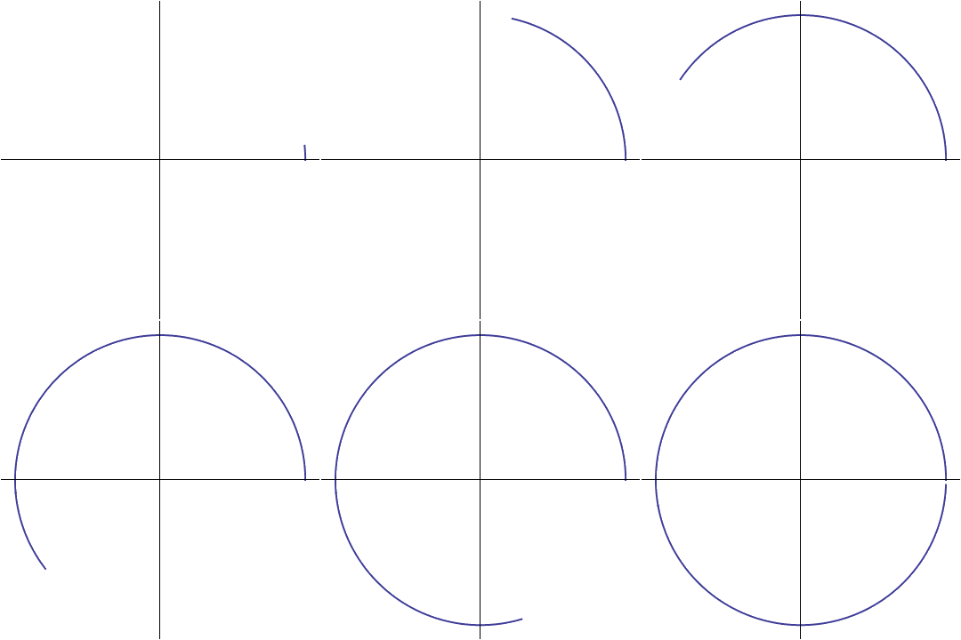High Frequency

Now what about the initial phase? The initial phase of a sinusoid just tells us where in the cycle to start: if the phase is zero we start on the positive x axis, and for any other phase we simply start from there: Initial phase: 0

Initial phase: 1

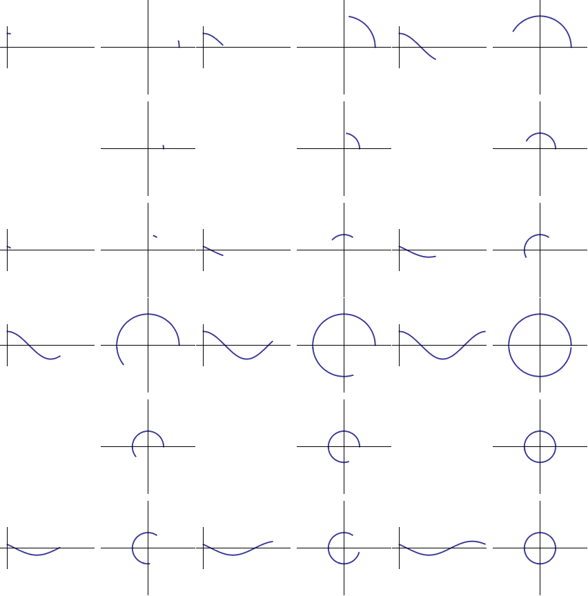
Ok, so we have figured out how to encode the frequency and the initial phase of a sinusoid by just choosing a different starting point and angular velocity to traverse the circle corresponding to the amplitude. From our model, we can read off all the information we wanted originally: $amplitude \to circle \; radius$ $frequency \to angular \; velocity$ $initial \; phase \to starting \; point$ There's only one thing missing: where are the complex numbers? Everything so far has been done in terms of plane geometry, and it seems rather useless. We replaced a sinusoid by a rotating point, so what? We managed to combine all three pieces of information into one picture, but not into one number: representing points in the plane requires two real coordinates. Here, finally, after constructing our entire model, we are ready to introduce the complex numbers. I presented it this way to try and emphasize the fact that there is nothing actually "imaginary" going on in this model, indeed the model can be constructed without them completely, just in terms of geometry! We have modeled our sinusoid as rotation on a circle, and this just so happens to be exactly what complex numbers do! That is, to use the complex numbers we are going to have to add one more map to our model $sinusoid \to plane\;geometry \to complex\;numbers$ Where the first step of this map was detailed above, and the second step is derived in detail in the article Exponentials: Discrete, Real, and Imaginary. In short, the complex numbers present us with an alternative to polar coordinates, and to parametrizing circles. To model a unit speed parametrization of the unit circle starting along the positive x axis, can write the complex expression $e^{it}$

If instead we want a unit angular speed parametrization of a circle of radius r, we can write the complex expression $r\cdot e^{it}$

And, if we want to traverse the circle at angular speed $\omega$ , we can write $r\cdot e^{i\omega t}$

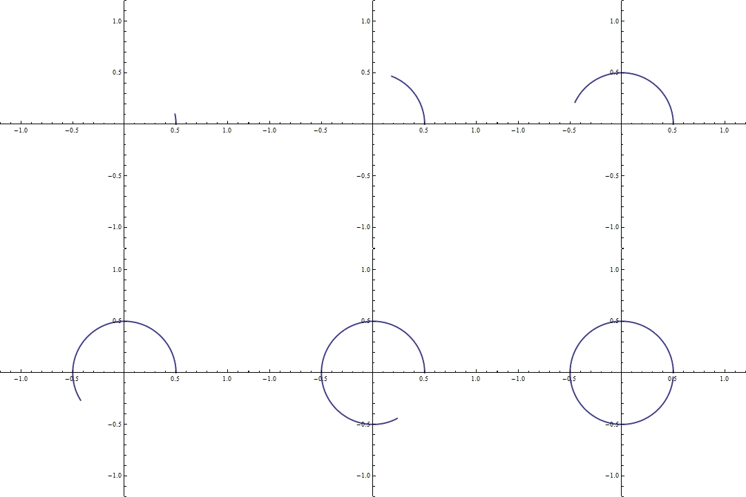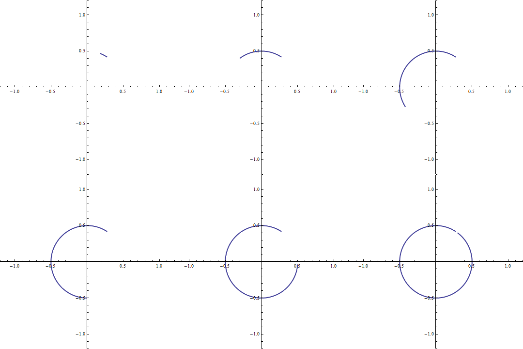A positive rotation of $\theta$ can be written $e^{i\theta}$ , and thus starting a rotation at angle $\theta$ from the horizontal can be modeled by multiplying the above exponential by $e^{i\theta}$ . $r\cdot e^{i\omega t}\cdot e^{i\theta}$

We then have our general expression which relates the formalism of complex numbers to our geometric model: $A\cdot e^{i\omega t}\cdot e^{i\theta_0}=(amplitude) \cdot e^{i\cdot (frequency) \cdot (time)}\cdot e^{i\cdot (initial\;phase)}$
$=circle\;of\;radius\;(A)\;traversed\;at\;speed\;(\omega)\;starting\; at \;(\theta_0)$ Using the complex numbers, we have managed to put the amplitude and phase of our oscillation into a single number, and we have a rather simple expression for its time dependence to boot! This is the reason the complex numbers have made their entrance: instead of lying along a line, they span a plane. Thus, they can encode two pieces of information at once. We decided to look at the plane as a collection of nested circles, and so our two coordinates were radius and phase. The polar form of complex numbers has an identical representation, so the model carried over nicely. Now we have our model, and the above equation gives us a way to transfer an oscillation into a complex exponential. But what about going the other direction? At the end of our work, we would like to get back to the real world, to interpret our result. In fact, it turns out that if we project our rotating point on the circle down onto the x-axis, we get our the representation of our original oscillation in terms of the cosine function! This is covered in more detail in Exponentials: Discrete, Real, and Imaginary, but we can project our rotating circle onto both the horizontal and vertical axes simultaneously by using euler's formula: $Ae^{i\omega t}e^{i\theta_0}=Ae^{i(\omega t+\theta_0)}=A\cos(\omega t+\theta_0)+i\cdot A\sin(\omega t +\theta_0)$

Thus the real part of our exponential is the representation of this wave with respect to the cosine as a base. This is what "taking the real part" of an expression does at the end of a long calculation; it gives us the oscillation form of our equation. What makes this model useful? Well, like the simpler models we talked about, once you map everything over to the model, you no longer have to worry about where the information came from, you can just manipulate the terms in the model and convert back when you are done. Lets look at a quick example: Say you want to model a process which takes in an oscillation, and phase shifts it by $\phi$ . If we can find a corresponding operation in our model which will accomplish this, then we can perform the following:

As we can see above, the "reverse map" back to the world of oscillations is performed by taking the horizontal projection of our rotating plane vector. So, what operation on a plane vector would cause a phase shift? Well, this is nothing different than our inclusion of an initial phase previously; we just need to move the vector $\phi$ radians before we rotate it; and this is symbolized by multiplication by $e^{i\phi}$ . This gives us

How about another process, like say we would like to model a device which changes the amplitude of a sinusoid by a factor of r. We know that after mapping the sinusoid to our model, its amplitude is represented by the length of the rotating vector. Changing the length of this vector can be done by a scaling transformation; multiplication by a scalar. This allows us to write

Putting these together, we can model a simultaneous change of phase and amplitude.

Here's the pictorial representation of the above schematic:

An example of this transformation is impedance in AC circuits. Say we have some AC circuit with a sinusoidally varying current. Using the base oscillation as a cosine, we know we can describe it with an amplitude, frequency, and an initial phase. In our model this translates to the rotating vector $I(t)=I_0\ \cdot e^{i\omega t}\cdot e^{i\theta_I}$

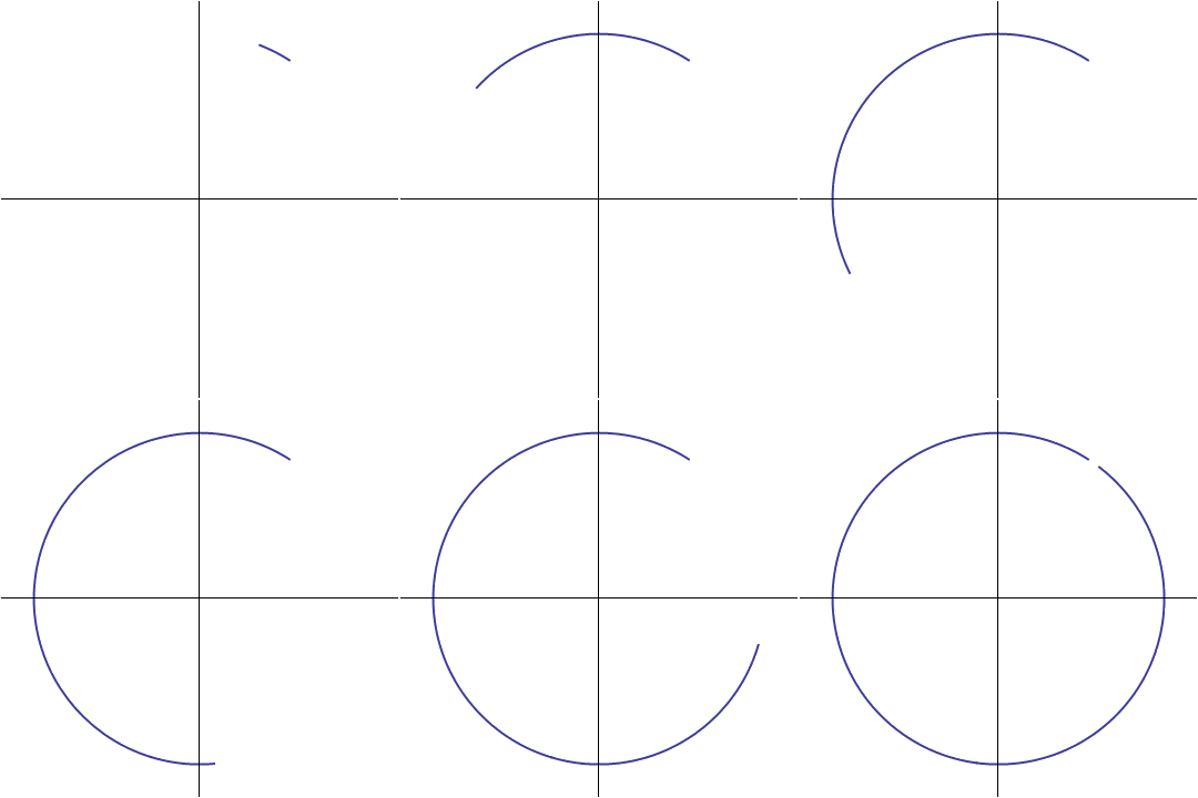Now, in our circuit we also have a voltage, which can be measured and turns out to be a sinusoid of the same frequency. In our model, this means voltage can be represented by a vector rotating at the same speed as the current vector, but possibly a different amplitude and phase. $V(t)=V_0\cdot e^{i\omega t}\cdot e^{i\theta_V}$

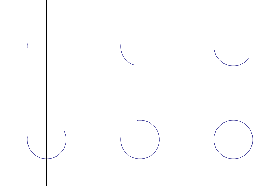This means the voltage and current vectors can only differ by two things: their length, and the position at which they begin their rotation. Lets say that the ratio of the voltage vector's length to the current vector's is R, and that it starts its rotation at an angle $\phi$ . Thus, we can say the voltage in our circuit is a stretched, shifted version of our current.

$voltage=current(stretched\;by\;R,\;rotated \;by\;\phi)$ In our model, we can represent a stretch by R by scalar multiplication, and a rotation by $\phi$ with multiplication by $e^{i\phi}$ . Thus, the above verbal equation can be re-expressed algebraically in the model: $V=I\cdot R\cdot e^{i\phi}$ The operator here, namely the command "stretch by R, rotate by $\phi$ " is concisely summed up by two multiplications. Applying these two multiplications in succession is equivelant to just a multiplication by $Z=R\cdot e^{i\phi}$ , which lets us write the relationship of voltage to current in the following way: $V=I\cdot Z$ Where Z is typically called the impedance. However, thinking about its origin within our model, we see that impedance is simply a way to describe the "stretch and shift" which relates voltage to current. Another useful feature of our rotating vector model is the ease with which we can add sinusoids. Let's say we are given two oscillations at the same frequency, but with different amplitudes and phase shifts:

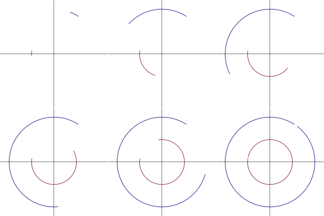
Now say we want to superpose (add) them to get a third sinusoid. We could do this in oscillation-land by taking the value of each point along the horizontal axis and adding them, to produce a third wave (the gold curve in the figure below)

But, this is not particularly instructive, and gives no intuition (other than the fact that the value of the new sinusoid at any given point is the sum of the two others, but that is pretty obvious). Instead, look what happens if we convert each of the original sinusoids to our model first. We can look at each as being a rotating vector in the plane, moving at the same speed but with different lengths, and offset from each other by an angle. The sum of the two sinusoids can then be accomplished by vector addition (the parallelogram rule), which intuitively gives us a new vector rotating at the same speed, but at a different angle and of different length than either of the inputs. When we are done adding, we can just project on the horizontal axis to get our resultant wave:

Personally, I find this way of thinking about the superposition of oscillations to be much more intuitive, and easier to "see whats going on" in your head without actually performing the computation. For instance, since the two vectors are rotating at the same speed, their sum will obviously rotate at that speed as well; and so we can see that the sum of two sinusoids sharing one frequency will also have that frequency. Looking at the first plot in this section, the two terms of the summand, its not nearly as apparent that their sum will be sinusoidal, much less one of the same frequency. The modeling of oscillations with complex numbers has a three part structure; as discussed before. First, we identify the important parts of each oscillation with a rotation in the plane, and then we express that rotation with the complex numbers. The mapping of the various operations discussed above are presented here schematically, as a refresher. Note the three-tier structure to each. $sinusoids \to plane \; geometry \to complex\;numbers$ $oscillation\to\;rotating\;point\;in\;the\;plane\to\;r\cdot e^{i\omega t+\theta}$ $phase\;shift\to\;rotation\;in\;the\;plane\to\;multiplication\;by\;e^{i\theta}$ $amplitude\;change\to\;radial\;stretch\;of\;plane\to \;multiplication\;by\;R$ $superposition \to vector \; addition \to (r_1 e^{i\theta_1}+r_2 e^{i\theta_2})e^{i\omega t}$ After doing all the calculations in the model, we can reclaim the resultant sinuosid with the reverse map $sinusoid\xleftarrow{horizontal \;projection} rotating\;point \xleftarrow{graphing}e^{i\omega t+\theta}$ Which is more commonly viewed as the the mapping $sinusoid\ \xleftarrow{real \;part}e^{i\omega t+\theta}$ Hopefully its apparent that the imaginary numbers are just a tool to help us express our model, and the real sneakiness lies in representing an oscillation with a planar rotation instead of a sinusoidal graph. Its much easier to deal with rotations than with a trigonometric curve, so as long as we preserve all the useful information (which I hope I've convinced you we have!), why not do it?

标签：will,Applications,Engineering,so,numbers,搬运,phase,our,model
来源： https://www.cnblogs.com/heweiren-cheng/p/14844105.html