Exploring Market Making Strategy for High Frequency Trading: An Agent-Based Approach

https://link.springer.com/chapter/10.1007/978-3-319-20591-5_6

Abstract

This paper utilizes agent-based simulation to explore market making strategy for high frequency traders (HFTs) and tests its performance under competition environments. After proposing a model representing HFTs’ activities in financial market when they act as market makers, we carry out simulations to explore how order price and order quantity affect HFTs’ profits and risks. As the result, we find that offering prices around last trading price, as well as taking advantage of order imbalance, increases HFTs’ returns. On the other hand, our results show utilizing adaptive order size based on previous order execution rate and setting a net threshold based on average trading volume helps to control the risks of end-of-day inventory. In addition, we introduce the competition environments of increased competitors and decreased latency, so as to see how these factors affect the performance of market making strategy.

Keywords

Order Quantity Market Making Total Return Trading Price Tick Size  These keywords were added by machine and not by the authors. This process is experimental and the keywords may be updated as the learning algorithm improves. Download conference paper PDF

6.1 Introduction

On March 11th, 2014, Virtu Financial Inc., the high frequency market maker, who had just one day of trading losses in 1238 days, filed for an initial public offering. Many people were astonished by their near-perfect record as a market maker, while others argued that the profit is becoming unsustainable due to competitions. In this paper we address two questions: what kind of market making strategy helps to increase HFTs’ profit, and how this strategy performances under competition environments?

The Securities and Exchange Commission (SEC) generalized four types of trading strategies that often utilized by HFTs [1]. Among them, market making is the most transparent one and constitutes more than 60 % of HFT volume [2]. Menkveld carefully studied the profits and net position of a large HFT who acts as a modern market maker [3]. But the strategies under the performance of this HFT, as well as the relationship between strategy and market condition, remains unrevealed.

The formidable challenge for better revealing HFT activities, is obtaining comprehensive and detailed data. Agent-based simulation provides an effective way to solve this problem, and has already been used to design trading strategies. Kendall and Su use an agent-based model to evolve successful trading strategies by integrating individual learning and social learning [4]. Nevmyvaka et al. use a simple class of non-predictive trading strategies to test electronic market making, and examine the impact of various parameters on the market maker’s performance [5]. Wang et al. implement a learning algorithm for market makers to search the optimal trading frequency, and they study how different trading frequencies of market makers affect the market [6]. Wah and Wellman employ simulation based methods to evaluate heuristic strategies for market makers and find the presence of the market maker is benefit to both impatient investors and overall market [7]. Comparing with their approaches, our agent-based simulation focuses on testing the combinations of different classes of market making strategies for HFTs, and further examining the performance in competitive environments. Our main contributions are as follows:

• We build an artificial transaction system to represent HFTs’ activities in stock market when they act as market makers. This system fits with main statistical properties of financial markets and is used to compare the performance of different market making strategies.

• We find one market making strategy which increases daily return and decreases end-of-day inventory, is offering prices around last trading price, as well as take advantage of order imbalance, together using adaptive order size based on previous order execution rate and a net threshold based on average trading volume.

• We further introducing the environment of increased competitors and decreased latency, in order to test the strategy under different market conditions.

6.2 Modelling of High Frequency Trading

In this section, we propose an artificial stock market in which agents trade through a limit-order book (LOB). Agents are classified into two categories according to their goals and strategies. The one is Low Frequency Traders (LFTs), who concern the value of the asset and try to earn the profit using an integrated strategy of fundamentalist and chartist. The other is High Frequency Traders (HFTs), who ignore the value of the asset but only pay attention to the trading environment itself, and they mainly try to accumulate the profit on the spread using the market making strategy. We stimulate the intra-day transaction scenario where both agents trade on one single asset. The framework of the model are presented first, following by details.

6.2.1 Framework

The model is an extension of the one presented by Leal et al. [8]. There are totally T sessions in each of which both HFTs and LFTs trade. The trading procedure is as follows:

1. 1.

   Active LFTs decide whether to enter the market according to their expected returns. If enter, they submit either a sell or a buy order with size and price based on their expectations.

    
2. 2.

   Knowing the orders submitted by LFTs, HFTs decide whether to enter the market. If enter, they usually submit both a sell and a buy order with size and price in order to absorb the orders of LFTs and earn the profit on the spread.

    
3. 3.

   LFTs and HFTs’ orders are matched and executed according to their price and arrival time. the last trading price is determined then and unexecuted orders rest in the LOB for the next trading session.

    
4. 4.

   After each session, LFTs and HFTs decide whether to update their trading parameters according to their performances.

    

6.2.2 Low Frequency Traders Activity

For each trading session, LFT i acts as following:

1. 1.

   Decides whether to be active according to its active possibility LFi_apLFi_ap.

   LFi_apLFi_ap is drawn from a uniform distribution with support [αLmin,αLmax][αminL,αmaxL] and may be changed according to individual profit.

    
2. 2.

   If being active, LFT i first calculates the expected price of the asset LFi_EPLFi_EP based on its expected return LFi_ERLFi_ER, then generates the ask price LFi_APtLFi_APt and bid price LFi_BPtLFi_BPt at time t based on last trading price p t .

   The return at time t are defined as Rt=log(ptpt−1)Rt=log(ptpt−1) (6.1) Utilizing the idea of LeBaron and Yamamoto [9]. LFTs form their weighted forecasts on the future returns by combining fundamental-, chart-, and noise-based forecasts as follows: LFi_ER=ni1×log(pfpt)+ni2×1li∑j=1lilog(pt−1pt−j−1)+ni3×N(0,1)LFi_ER=n1i×log(pfpt)+n2i×1li∑j=1lilog(pt−1pt−j−1)+n3i×N(0,1) (6.2) and the expected price LFi_EPLFi_EP is calculated as pt×eLFi_ERpt×eLFi_ER.

   l i represents the memory length of LFT i, and li∼U(1,lmax)li∼U(1,lmax). ni1n1i, ni2n2i, ni3n3i are weights for fundamentalist, chartist, and noise-induced components for LFT i, respectively, and randomly assigned according to normal distributions: ni1∼|N(0,σ1)|n1i∼|N(0,σ1)|, n2 i  ∼ N(0, σ2), and ni3∼N(0,σ3)n3i∼N(0,σ3).

   And price for sell/buy orders at time t are formed as follows: LFi_APt=pt−1×(1−κiL)LFi_BPt=pt−1×(1+κiL) (6.3) where κi∼U(κmin,κmax)κi∼U(κmin,κmax) represents the price fluctuation parameter.  
3. 3.

   If the ask price of LFT i is higher than its expected future price, LFT i will submit a sell order at price LFi_APtLFi_APt with size LFi_ASLFi_AS; if the bid price of LFT i is lower than its expected future price, it will submit a buy order at price LFi_BPtLFi_BPt with size LFi_BSLFi_BS. The valid time of the order is γLγL.

   The size of the orders are proportional to expected returns and are formed as: LFi_AS=LFi_ER×ηiLLFi_BS=−LFi_ER×ηiL (6.4) where ηLiηiL represents the size fluctuation parameter of LFTs and ηLi∼U(ηLmin,ηLmax)ηiL∼U(ηminL,ηmaxL), it can be changed according to individual profit. And if the order has not been fully executed within γ L , the rest of it will be removed from the LOB.  
4. 4.

   After τ sessions, LFT i decide whether to update its trading parameters based on its profit LFi_PtLFi_Pt.

   if LFi_Pt>0LFi_Pt>0, LFT i will update some of its parameters as:

   LFi_ap∼U(LFi_ap,αmax)LFi_ap∼U(LFi_ap,αmax) ηLi∼U(ηLi,ηLmax)ηiL∼U(ηiL,ηmaxL)

   if LFi_Pt⩽0LFi_Pt⩽0, it becomes:

   LFi_ap∼U(αmin,LFi_ap)LFi_ap∼U(αmin,LFi_ap) ηLi∼U(ηLmin,ηLi)ηiL∼U(ηminL,ηiL)

   if LFi_Pt⩽0LFi_Pt⩽0 and a random number ∼U[0,1]<λ∼U[0,1]<λ, then the component-weighted parameters and memory length will be renewed based on the distributions:

   ni1∼|N(0,σ1)|n1i∼|N(0,σ1)|, ni2∼N(0,σ2)n2i∼N(0,σ2), ni3∼N(0,σ3)n3i∼N(0,σ3), and li∼U(1,lmax)li∼U(1,lmax).

    

6.2.3 High Frequency Traders Activity

For each trading session, HFT j acts as follows:

1. 1.

   HFT j decides whether to be active based on the price fluctuation PflutPtflu (bps) at time t and its action threshold HFj_atHFj_at.

   Since evidence suggests HFT activities prefer higher volatility. We calculate Pflut=|pt−1−pt−2pt−1|×10,000Ptflu=|pt−1−pt−2pt−1|×10,000 (6.5) and HFj_at∼U(αHmin,αHmax)HFj_at∼U(αminH,αmaxH). If Pflut>HFj_atPtflu>HFj_at, then HFT j becomes active.  
2. 2.

   If being active, it submits both a sell order at price HFj_APHFj_AP with size HFj_ASHFj_AS and a buy order at price HFj_BPHFj_BP with size HFj_BSHFj_BS. All orders from HFTs are submitted in a random order, and the valid time of the orders is γ H .

   Under the defaulted setting, HFj_AP=pt+κHjHFj_AP=pt+κjH, HFj_BP=pt−κHjHFj_BP=pt−κjH, κ H refers to price fluctuation. While HFTs decide the order quantity based on the quotes in the LOB. HFj_AS=HFj_BS=0.5×(qb+qs)×ηHjHFj_AS=HFj_BS=0.5×(qb+qs)×ηjH. Where q b (q s ) refers to the total size of buy (sell) orders in the LOB at this session, and η H refers to order absorption rate.

    
3. 3.

   Like LFTs, after τ sessions, HFT j decide whether to update ηHjηjH based on its performance.

    

6.2.4 Model Validation

Table 6.1 lists the defaulted value of all the parameters. The number of sessions is set as 400 for intra-day trading. There are 441 traders, and 2 % (9) of them are HFTs [2]. Price and volume related parameters are calibrated to fit with market volatility and liquidity condition respectively, while keeping the diversity of agents. Table 6.1

Parameters in initial simulation

Description	Symbol	Defaulted
Number of trading sessions	T	400
Number of traders	N	441
Fundamental value	p f	50
Tick size	t s	0.01
LFT initial active possibility	[α min L , α max L ]	[0.01, 0.1]
LFT max memory length	l max	30
LFT order price fluctuation	[κ min L , κ max L ]	[−0.002, 0.01]
LFT order size fluctuation	[η min L , η max L ]	[200, 1000]
LFT order life	γ L	10
LFT parameter evolution circle	τ	30
LFT parameter evolution rate	λ	0.3
Std of fundamental component	σ 1	0.3
Std of chartists component	σ 2	0.6
Std of noise-trader component	σ 3	0.1
HFT percentage	HFT per	2 %
HFT active threshold	[α min H , α max H ]	[5, 5]
HFT order price fluctuation	κ H	0.01
HFT order absorption rate	[η min H , η max H ]	[0.1, 0.5]
HFT order life	γ H	1

We check whether the model is able to account for the main stylized facts of financial markets. The price movement generated by the model is in line with the empirical evidence as absence of autocorrelation, see as Fig. 6.1. In contrast, the autocorrelation function of absolute return display a slow decaying pattern, see as Fig. 6.2. In addition, the existence of fat tails in the distribution of price is shown in Fig. 6.3. 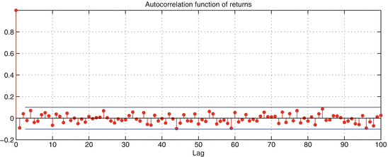Open image in new window Fig. 6.1

Autocorrelation of return in HFT simulations

Open image in new window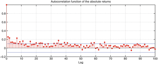 Fig. 6.2

Volatility clustering in HFT simulations

Open image in new window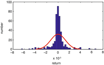 Fig. 6.3

Return distribution in HFT simulations

6.3 Exploration of Market Making Strategy

In this section, we design experiments concerning HFT order price, order quantity respectively, trying to find what kind of order price and order quantity help HFTs increasing profits and decreasing risks.

Based on [3], our model assumes HFTs usually utilize passive market making and try to earn the spread. But when they speculated order imbalance by detecting the transaction trends of LFTs, they may utilize aggressive market making. In this case they trade on quickly to get the profit from price movement, or close their position. In the model, we consider HFT’s profit as the daily return, and the risk as the end-of-day inventory. All transaction fees are ignored for simplicity.

6.3.1 Strategies for Order Price

HFTs switch between passive and aggressive market making. In usual case, HFT use passive market making as a liquidity maker, and they quote either based on last trading price or best ask/bid price to earn the spread. But when the volume difference between ask and bid quoting becomes significant, i.e. when |qb−qs|/(qb+qs)|qb−qs|/(qb+qs) is over a threshold, they will adopt aggressive market making. In this case HFTs will either quoting along with temporary trend to earn the profit based on the price movement, or against it to take liquidity in order to adjust their position. Shown as Fig. 6.4. Open image in new window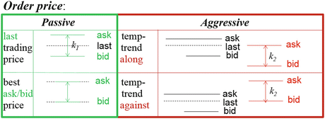 Fig. 6.4

Passive and aggressive market making

When HFTs adopt passive market making and offer price around the last trading price, the ask order is offered at p t + 0. 5 × k1 and bid order at p t − 0. 5 × k1, where k1 refers to the ask-bid spread in passive market making condition and its default value is twice the tick size. While offering price around the best ask/bid, they offer ask order at best ask and bid order at best bid in the LOB.

While setting the threshold as 0.5, we suppose when |qb−qs|/(qb+qs)>0.5|qb−qs|/(qb+qs)>0.5, HFTs will adopt aggressive market making. If sell orders is much more than buy orders, quoting along with the temporary trend means offering ask price at last trading price p t and bid price at p t − k2, where k2 refers to the ask/bid spread in aggressive market making condition. And quoting against with temporary trend means offering ask price at p t + k2 and bid price at p t .

6.3.2 Strategy for Order Quantity

Another question need to be discussed for the strategy is order quantity. In order to gain more profits and fewer risks, HFTs will consider two aspects, increasing the chance of order fulfillment and keeping flat position accordingly.

For the first aspect, When HFTs utilizes passive market making, they are aiming to absorb the orders submitted by LFTs and earn the spread. And when HFTs use aggressive market making, they try to make profits base on the excess liquidity. All HFTs will adaptively adjust their order quantity by calculating the average order execution rate in past few sessions. Suppose r m and r h refer to the market order execution rate and self order execution rate in past τ sessions, so the order quantity Q is decide by: Passive:Q=min(qb,qs)×0.5×(rm+rh)Aggressive:Q=|qb−qs|×0.5×(rm+rh) (6.6) For the second aspect, based on the previous work by Menkveld and Hendershott [3, 10], we introduce a parameter named net threshold, denoted as NT to supervise the net position of HFTs, denoted as np. Suppose V i represents the trading volume in session i and NT is proportional to average trading volume in first τ periods, so after τ periods, NT is calculated and works as follows: NT=1τ∑i=1τViNT=1τ∑i=1τVi (6.7)

• When | np |  < 0. 5 × NT, it trades as usual.

• 0.5×NT⩽|np|<NT0.5×NT⩽|np|<NT, it applies price pressure and adjusts its quotes by one tick size.

• When |np|⩾NT|np|⩾NT, it stops one side (buy or sell) trading.

• a HFT’s max order size equals NT.

6.3.3 Comparison of Strategies

In last two sections, we mentioned the strategies used for passive and aggressive market making, as well as the method to control end-of-day inventory. We suppose HFTs can use either single or combination of market making, so totally eight types of quoting methods are list in Table 6.2. Table 6.2

List of quoting strategies

Strategy	Market conditions
	(qb−qs)/(qb+qs)>0.5(qb−qs)/(qb+qs)>0.5		(qs−qb)/(qb+qs)>0.5(qs−qb)/(qb+qs)>0.5		Other
	ask price	bid price	ask price	bid price	ask price	bid price
last trading	p t + 0. 5 × k1	p t − 0. 5 × k1	p t + 0. 5 × k1	p t − 0. 5 × k1	p t + 0. 5 × k1	p t − 0. 5 × k1
green1ask/bid	best ask	best bid	best ask	best bid	best ask	best bid
trend-along	p t + k2	p t	p t	p t − k2	NA	NA
trend-against	p t	p t − k2	p t + k2	p t	NA	NA
red1last+along	p t + k2	p t	p t	p t − k2	p t + 0. 5 × k1	p t − 0. 5 × k1
last+against	p t	p t − k2	p t + k2	p t	p t + 0. 5 × k1	p t − 0. 5 × k1
ask/bid+along	p t + k2	p t	p t	p t − k2	best ask	best bid
ask/bid+against	p t	p t − k2	p t + k2	p t	best ask	best bid

Supposing 2 % of the traders are HFTs, all of them use a same quoting strategy, selected from the list, together with adaptive order quantity and net threshold for controlling inventory, and their orders are submitted in a random order. We test the performance of these strategies focused on the daily return and end-of-day inventory, denoted as EDI. After testing each strategy for 250 simulations, Fig. 6.5 shows the average return and inventory of these strategies. 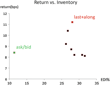EDI%=|np|NT×100%EDI%=|np|NT×100% (6.8) Open image in new window Fig. 6.5

Comparison of different market making strategies

According to the graph, we see that quoting based on best ask/bid price has its advantage on inventory, which indicate this strategy has the lowest risk. While quoting based on last trading price together using a temporary trend along strategy, lead to the highest return for HFTs. Here, we choose the last+along strategy as the benchmark for further experiments.

6.4 Experiments on Competition

In following simulations, we change the percentage of HFTs (2 % in previous experiments) to see its influence. On the other hand, all HFTs submit their orders in a random order in past experiments, which means they have similar latencies. Considering HFTs are pursuing lower latency in order to run in front of their competitors nowadays, we arrange different latencies for HFTs. In this case HFTs submit their orders one after another in a fixed order, thus a HFT with lower latency submits its orders earlier and is likely to have higher order execution probabilities.

6.4.1 Total Return of HFTs

We first consider the total return of HFTs. We concern how HFTs’ profit will be affected by increased competitors and decreased latency. While all HFTs using the last+along strategy, we adjust the number of HFTs, and run the simulation 250 times for each different HFT percentage (0.5 %, 1 %, 1.5 %, …5 %) first in similar then in different latency settings. The total return of HFTs is calculated and shown in Fig. 6.6: Open image in new window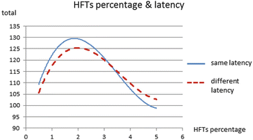 Fig. 6.6

Total return of HFTs

There are two things interesting according to this result. On one hand, in both latency conditions, the total return of HFTs first went up and then down. This may because when the number of HFTs is small, HFTs do not fully absorb LFTs’ orders and there are still surplus profit on the spread. But when this number becomes larger, HFTs suffer from position imbalance and need to pay the price to trade out of their positions, thus causes a decline in their total return. On the other hand, the red curve shows the condition that HFTs compete with each other on speed and have different latencies. Comparing to the blue one, it indicates this competition actually decreases HFTs’ total return when the number of HFTs is small but increases their total return when the number is larger.

6.4.2 Individual Return of HFTs

We then turn to the individual return of HFT and concern the value of low-latency. Supposing HFTs have different latencies, Fig. 6.7 depicts the return difference among LFTs, normal HFTs and the fastest HFT. Open image in new window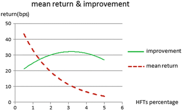 Fig. 6.7

Individual return of HFTs

In the result, the red curve shows the average individual return of HFTs, it decreases with the increase of HFTs percentage and can be seen as the return of a normal HFT. Since LFTs’ population is much more than HFTs’ and their average return can be seen as zero, the red curve also illustrates the return difference between a normal HFT and a LFT approximately, and can be taken as a reference for a LFT to decide whether it is worth taking part in HFT. The green curve, on the other hand, is calculated as the difference between the average and the highest return (return of the HFT with the lowest latency). It can be interpreted as how much potential profit can be earned for a normal HFT to become the fastest one by renewing its devices or using co-location method. This chart may suggest that although the profit for becoming a HFT decreases with the increase of HFTs, it is always profitable for a HFT to pursue lower latency.

6.5 Conclusions

This paper focuses on exploring market making strategy for High Frequency Trading and consists of three parts. First we combine previous work and build an intra-day transaction model based on limit order book to simulate the trading activities of HFTs and LFTs. In addition, by analyzing both passive and aggressive market making, we try to figure out what kind of order price and order quantity help HFTs increasing their profits and decreasing their risks. Finally, we test the strategy in competition environments including increased competitors and decreased latency, in order to see its performance.

References

1. 1. Securities and Exchange Commission (2010) Fed Reg 75(13):3594Google Scholar
2. 2. Hagströmer B, Nordén L (2013) J Financ Mark 16(4):741CrossRefGoogle Scholar
3. 3. Menkveld AJ (2013) J Financ Mark 16(4):712CrossRefGoogle Scholar
4. 4. Kendall G, Su Y (2003) Proceedings of IEEE, pp 2298–2305Google Scholar
5. 5. Nevmyvaka Y, Sycara K, Seppi D (2003) In: Proceedings of the third international workshop on computational intelligence in economics and financeGoogle Scholar
6. 6. Wang C, Izumi K, Mizuta T, Yoshimura S (2013) SICE J Control Meas Syst Integr 6(3):216CrossRefADSGoogle Scholar
7. 7. Wah E, Wellman MP (2015) In: Fourteenth international conference on autonomous agents and multi-agent systemsGoogle Scholar
8. 8. Jacob Leal S, Napoletano M, Roventini A, Fagiolo G (2014) Rock around the clock: an agent-based model of low-and high-frequency trading. Technical Report, Groupe de REcherche en Droit, Économie, Gestion (GREDEG CNRS), University of Nice Sophia AntipolisGoogle Scholar
9. 9. LeBaron B, Yamamoto R (2007) Phys A: Stat Mech Appl 383(1):85MathSciNetCrossRefGoogle Scholar
10. 10. Hendershott T, Menkveld AJ (2010) Price pressures. Technical Report, CFS Working PaperGoogle Scholar

标签：Exploring,Based,price,HFT,Agent,order,trading,HFTs,market
来源： https://www.cnblogs.com/dhcn/p/14446419.html