首页 > 其他分享> > 自适应波束合成

自适应波束合成

2022-01-14 16:33:20 作者：互联网

自适应波束合成的自适应三个字体现在针对不同数据，波束的合成不仅对期望方向有增益，还对干扰方向有一定的抑制。

信号数据

因为都要计算自相关矩阵，而不同的信号之间应该是非相干的，噪声之间也是非相干的。所以可以直接用随机数代替信号。并且由于采样率和信号频率之间只决定了快拍数，而信号频率假设已知(因为要计算理想情况下的 d = λ 2 d=\frac{\lambda}{2} d=2λ)，所以采样率也忽略了。如果认为噪声的信号为单位1，则信号的功率也为1，所以需要根据snr反算信号的幅度 A s A_s As，得到接收信号。

M = 40;
c = 3e8;
N=300;
f = 4.5*1e6;
lambda = c./f;
SNR = [0, 30, 40];
R_circ = 175;
thetaK = [50, 20, 40]/180*pi;
phiK = [120, 240, 140]/180*pi;         
As = 10.^(SNR./20); 
A = [exp(1i*2*pi/lambda*R_circ*sin(thetaK(1))*cos(phiK(1)-2*pi*(0:M-1)/M));exp(1i*2*pi/lambda*R_circ*sin(thetaK(2))*cos(phiK(2)-2*pi*(0:M-1)/M));exp(1i*2*pi/lambda*R_circ*sin(thetaK(3))*cos(phiK(3)-2*pi*(0:M-1)/M))].';
signal=randn(length(thetaK),N);
for i=1:1:length(SNR)
    signal(i, :) = signal(i, :)*As(i);
end
noise = (randn(M, N)+1i*randn(M, N))/sqrt(2);
xn = A*signal+noise;

算法实现

MVDR

原理导出都有，简单的说就是使期望方向增益不变的前提下，总功率最小的。

R = xn*xn'/N;
expect_n=1;
noise_n=2;
noise_nn=3;
A_expect = A(:, expect_n);
w0 = inv(R)*A_expect/(A_expect'*inv(R)*A_expect);

dis = 1;
theta_scan = (0:dis:90-1)/180*pi;
phi_scan = (0:dis:360-1)/180*pi;


F = zeros(length(theta_scan), length(phi_scan));
for i=1:length(theta_scan)
    for j=1:length(phi_scan)
        a = exp(1i*2*pi/lambda(expect_n)*R_circ*sin(theta_scan(i))*cos(phi_scan(j)-2*pi*(0:M-1)/M).');
        F(i, j) = w0'*a;
    end
end
F_abs = 20*log(abs(F));

MVDR_1 MVDR_2

LCMV_1 LCMV_2

LCMV

LCMV是MVDR的直接扩展，由一个约束变为多个约束，将约束条件变为让多个方向（一个也可以）的增益不变，另外的干扰方向的增益为0。

M = 40;
c = 3e8;
N=300;
f = 4.5*1e6;
lambda = c./f;
SNR = [0, 30, 40];
R_circ = 175;
thetaK = [50, 20, 40]/180*pi;
phiK = [120, 240, 140]/180*pi;         
As = 10.^(SNR./20); 
A = [exp(1i*2*pi/lambda*R_circ*sin(thetaK(1))*cos(phiK(1)-2*pi*(0:M-1)/M));exp(1i*2*pi/lambda*R_circ*sin(thetaK(2))*cos(phiK(2)-2*pi*(0:M-1)/M));exp(1i*2*pi/lambda*R_circ*sin(thetaK(3))*cos(phiK(3)-2*pi*(0:M-1)/M))].';
signal=randn(length(thetaK),N);
for i=1:1:length(SNR)
    signal(i, :) = signal(i, :)*As(i);
end
noise = (randn(M, N)+1i*randn(M, N))/sqrt(2);
xn = A*signal+noise;

R = xn*xn'/N;
dis = 1;
theta_scan = (0:dis:90-1)/180*pi;
phi_scan = (0:dis:360-1)/180*pi;
C_matrix = A;
matrix_f = [1,0,0].'; %约束向量
F = zeros(length(theta_scan), length(phi_scan));

w0 = inv(R)*C_matrix/(C_matrix'*inv(R)*C_matrix)*matrix_f;

for i=1:length(theta_scan)
    for j=1:length(phi_scan)
        a = exp(1i*2*pi/lambda(1)*R_circ* sin(theta_scan(i))*cos(phi_scan(j)-2*pi*(0:M-1)/M).');
        F(i, j) = w0'*a;
    end
end
F_abs = 20*log(abs(F));

RAB

RAB是鲁棒自适应波束合成，目的是通过导向矢量在信号-干扰子空间上的投影，得到一个更为精确的导向矢量。

M = 40;
c = 3e8;
N=300;
f = 4.5*1e6;
lambda = c./f;
SNR = [0, 30, 40];
R_circ = 175;
thetaK = [50, 20, 40]/180*pi;
phiK = [120, 240, 140]/180*pi;         
As = 10.^(SNR./20); 
A = [exp(1i*2*pi/lambda*R_circ*sin(thetaK(1))*cos(phiK(1)-2*pi*(0:M-1)/M));exp(1i*2*pi/lambda*R_circ*sin(thetaK(2))*cos(phiK(2)-2*pi*(0:M-1)/M));exp(1i*2*pi/lambda*R_circ*sin(thetaK(3))*cos(phiK(3)-2*pi*(0:M-1)/M))].';
signal=randn(length(thetaK),N);
for i=1:1:length(SNR)
    signal(i, :) = signal(i, :)*As(i);
end
noise = (randn(M, N)+1i*randn(M, N))/sqrt(2);
xn = A*signal+noise;
R = xn*xn'/N;
dis = 1;% 扫描间隔
theta_scan = (0:dis:90-1)/180*pi;
phi_scan = (0:dis:360-1)/180*pi;

[E_all, lambda_all] = eig(R) ;
Es = E_all(:, end:-1:end-length(thetaK)+1);
C_matrix = A(:, 1);
F = zeros(length(theta_scan), length(phi_scan));
C_matrix = Es*Es'*C_matrix;
w0 = inv(R)*C_matrix/(C_matrix'*inv(R)*C_matrix);

for i=1:length(theta_scan)
    for j=1:length(phi_scan)
        a = exp(1i*2*pi/lambda(1)*R_circ*sin(theta_scan(i))*cos(phi_scan(j)-2*pi*(0:M-1)/M).');
        F(i, j) = w0'*a;
    end
end

F_abs = 20*log(abs(F));

画图

%% 画图
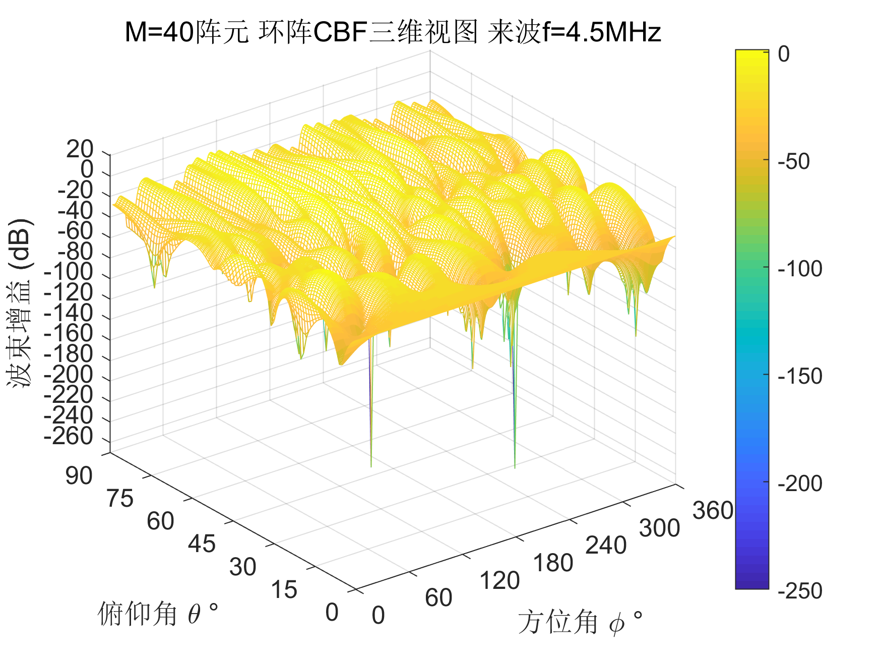
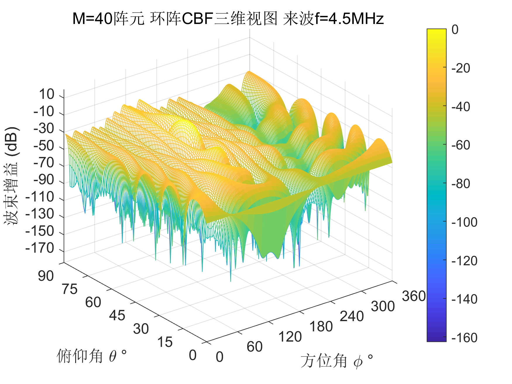
figure(1)
mesh(phi_scan*180/pi,theta_scan*180/pi,F_abs)
colorbar;
xlabel('方位角 \phi °');
ylabel('俯仰角 \theta ° ');
zlabel('波束增益 (dB)');
title(['M=',num2str(M),'阵元 环阵CBF三维视图 来波f=',num2str(f/1e6),'MHz']);
set(gca,'fontsize',12);
axis([0 360 0 90 min(min(F_abs))-20 max(max(F_abs))+20])
set(gca,'XTick',0:60:360);
set(gca,'YTick',0:15:90);
set(gca,'ZTick',(round(min(min(F_abs))/10)*10-10):20:20);

expect_n=1;
noise_n=2;
noise_nn=3;
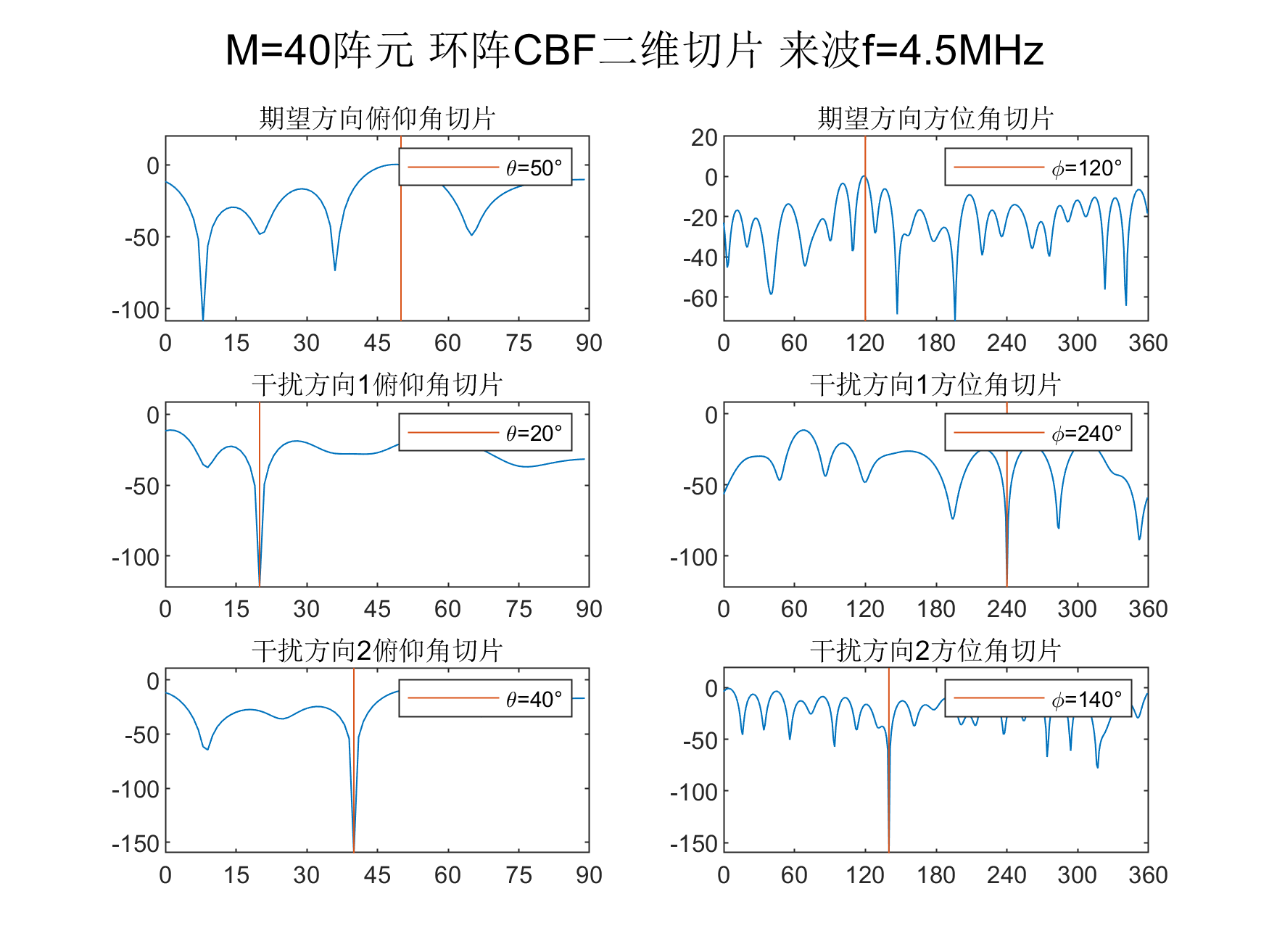
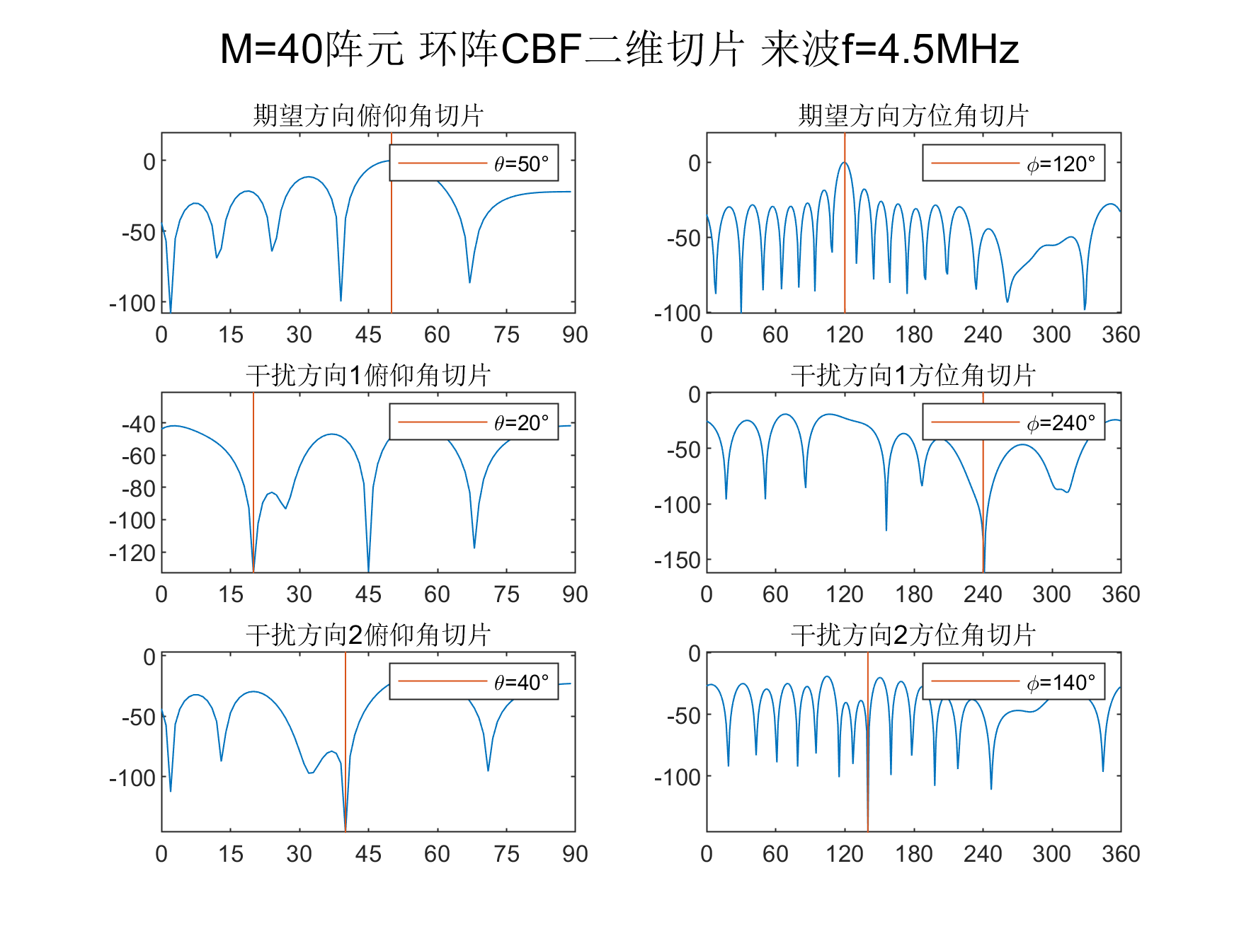
figure(2)
subplot(3,2,1)
plot(theta_scan*180/pi,F_abs(:, phi_scan==phiK(expect_n)),  'HandleVisibility', 'off')
hold on;
plot([thetaK(expect_n)/pi*180, thetaK(expect_n)/pi*180], [min(F_abs(:,phi_scan==phiK(expect_n))),40])
hold off;
title('期望方向俯仰角切片')
axis([0 90 min(F_abs(:,phi_scan==phiK(expect_n))) max(F_abs(:,phi_scan==phiK(expect_n)))+20])
set(gca,'XTick',0:15:90);
legend(['\theta=',num2str(thetaK(expect_n)/pi*180),'°']);

subplot(3,2,2)
plot(phi_scan*180/pi,F_abs(theta_scan==thetaK(expect_n), :),  'HandleVisibility', 'off')
hold on;
plot([phiK(expect_n)/pi*180, phiK(expect_n)/pi*180], [min(F_abs(theta_scan==thetaK(expect_n), :)),40])
hold off;
title('期望方向方位角切片')
axis([0 360 min(F_abs(theta_scan==thetaK(expect_n), :)) max(F_abs(theta_scan==thetaK(expect_n), :))+20])
set(gca,'XTick',0:60:360);
legend(['\phi=',num2str(phiK(expect_n)/pi*180),'°']);


subplot(3,2,3)
plot(theta_scan*180/pi,F_abs(:,phi_scan==phiK(noise_n)), 'HandleVisibility', 'off')
hold on;
plot([thetaK(noise_n)/pi*180, thetaK(noise_n)/pi*180], [min(F_abs(:,phi_scan==phiK(noise_n))),40])
hold off;
title('干扰方向1俯仰角切片')
axis([0 90 min(F_abs(:,phi_scan==phiK(noise_n))) max(F_abs(:,phi_scan==phiK(noise_n)))+20])
set(gca,'XTick',0:15:90);
legend(['\theta=',num2str(thetaK(noise_n)/pi*180),'°']);

subplot(3,2,4)
plot(phi_scan*180/pi,F_abs(theta_scan==thetaK(noise_n), :), 'HandleVisibility', 'off')
hold on;
plot([phiK(noise_n)/pi*180, phiK(noise_n)/pi*180], [min(F_abs(theta_scan==thetaK(noise_n), :)),40])
hold off;
title('干扰方向1方位角切片')
axis([0 360 min(F_abs(theta_scan==thetaK(noise_n), :)) max(F_abs(theta_scan==thetaK(noise_n), :))+20])
set(gca,'XTick',0:60:360);
legend(['\phi=',num2str(phiK(noise_n)/pi*180),'°']);

subplot(3,2,5)
plot(theta_scan*180/pi,F_abs(:,phi_scan==phiK(noise_nn)), 'HandleVisibility', 'off')
hold on;
plot([thetaK(noise_nn)/pi*180, thetaK(noise_nn)/pi*180], [min(F_abs(:,phi_scan==phiK(noise_nn))),40])
hold off;
title('干扰方向2俯仰角切片')
axis([0 90 min(F_abs(:,phi_scan==phiK(noise_nn))) max(F_abs(:,phi_scan==phiK(noise_nn)))+20])
set(gca,'XTick',0:15:90);
legend(['\theta=',num2str(thetaK(noise_nn)/pi*180),'°']);

subplot(3,2,6)
plot(phi_scan*180/pi,F_abs(theta_scan==thetaK(noise_nn), :), 'HandleVisibility', 'off')
hold on;
plot([phiK(noise_nn)/pi*180, phiK(noise_nn)/pi*180], [min(F_abs(theta_scan==thetaK(noise_nn), :)),40])
hold off;
title('干扰方向2方位角切片')
axis([0 360 min(F_abs(theta_scan==thetaK(noise_nn), :)) max(F_abs(theta_scan==thetaK(noise_nn), :))+20])
set(gca,'XTick',0:60:360);
legend(['\phi=',num2str(phiK(noise_nn)/pi*180),'°']);
suptitle(['M=',num2str(M),'阵元 环阵CBF二维切片 来波f=', num2str(f(1)/1e6),'MHz'])

标签：波束,abs,scan,合成,适应,180,noise,thetaK,pi
来源： https://blog.csdn.net/qq_41380292/article/details/122496943