【机器学习】otto案例介绍
作者:互联网
Otto Group Product Classification Challenge
1. 背景介绍
奥托集团是世界上最⼤的电⼦商务公司之⼀,在20多个国家设有子公司。该公司每天都在世界各地销售数百万种产品, 所以对其产品根据性能合理的分类非常重要。
不过,在实际工作中,工作人员发现,许多相同的产品得到了不同的分类。本案例要求,你对奥拓集团的产品进行正确的分类。尽可能的提供分类的准确性。
链接:https://www.kaggle.com/c/otto-group-product-classification-challenge/overview
2. 数据集介绍
- 本案例中,数据集包含大约200,000种产品的93个特征。
- 其目的是建立⼀个能够区分otto公司主要产品类别的预测模型。
- 所有产品共被分成九个类别(例如时装,电子产品等)。
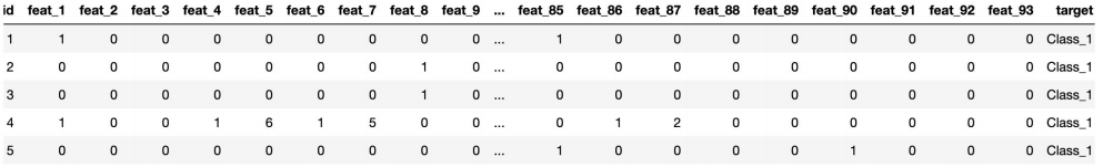
- id - 产品id
- feat_1, feat_2, …, feat_93 - 产品的各个特征
- target - 产品被划分的类别
3. 评分标准
本案例中,最后结果使⽤多分类对数损失进行评估。
具体公式:
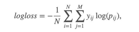
- i表示样本,j表示类别。Pij代表第i个样本属于类别j的概率,
- 如果第i个样本真的属于类别j,则yij等于1,否则为0。
- 根据上公式,假如你将所有的测试样本都正确分类,所有pij都是1,那每个log(pij)都是0,最终的logloss也是0。
- 假如第1个样本本来是属于1类别的,但是你给它的类别概率pij=0.1,那logloss就会累加上log(0.1)这⼀项。我们知 道这⼀项是负数,而且pij越小,负得越多,如果pij=0,将是无穷。这会导致这种情况:你分错了⼀个,logloss就是无穷。这当然不合理,为了避免这⼀情况,我们对非常小的值做如下处理:
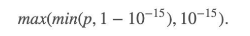
- 也就是说最小不会小于10^-15。
3.实现过程
- 获取数据
- 数据基本处理
- 数据量比较大,尝试是否可以进⾏数据分割
- 转换目标值表示方式
- 模型训练
- 模型基本训练
4. 数据获取
data = pd.read_csv('./data/otto/train.csv')

data.shape
(61878, 95)
data.describe()

图形可视化,查看数据分布
# 图形可视化,查看数据分布
import seaborn as sns

sns.countplot(data.target)

plt.show()

data.target

data.groupby(by='target').count()

5. 数据基本处理
数据已经经过脱敏,不需要特殊处理
5.1 截取部分数据
new_data = data[:10000]
使用上面截取不可行,然后使用随机欠采样获取相应的数据
# 随机欠采样获取数据
# 首先确定特征值/标签值

y = data['target']
x = data.drop(['id', 'target'], axis=1)  # axis=1按列删除

# 随机欠采样获取数据
from imblearn.under_sampling import RandomUnderSampler

rus = RandomUnderSampler(random_state=0)

x_resampled, y_resampled = rus.fit_resample(x, y)
x_resampled.shape, y_resampled.shape
((17361, 93), (17361,))
sns.countplot(y_resampled)

plt.show()

5.2 把标签值转换为数字
y_resampled.head()
0    Class_1
1    Class_1
2    Class_1
3    Class_1
4    Class_1
Name: target, dtype: object
from sklearn.preprocessing import LabelEncoder

le = LabelEncoder()

y_resampled = le.fit_transform(y_resampled)
y_resampled
array([0, 0, 0, ..., 8, 8, 8])
5.3 分割数据
from sklearn.model_selection import train_test_split

x_train, x_test, y_train, y_test = train_test_split(x_resampled, y_resampled, test_size=0.2)
x_train.shape, y_train.shape
((13888, 93), (13888,))
6. 模型训练
6.1 基本模型训练
from sklearn.ensemble import RandomForestClassifier

rf = RandomForestClassifier(oob_score=True)
rf.fit(x_train, y_train)
RandomForestClassifier(oob_score=True)
y_pre = rf.predict(x_test)
y_pre
array([0, 1, 6, ..., 6, 2, 1])
rf.score(x_test, y_test)
0.7857759861790958
rf.oob_score_  # 带外估计
0.7603686635944701
# 图形可视化,查看数据分布
import seaborn as sns

sns.countplot(y_pre)

plt.show()

# logloss模型评估
from sklearn.metrics import log_loss

log_loss(y_test, y_pre, eps=1e-15, normalize=True)

上面报错原因:logloss使用过程中,必须要求将输出用one-hot表示.
需要将这个多类别问题的输出结果通过One-HotEncoder修改如下:
y_test, y_pre
(array([0, 1, 6, ..., 6, 2, 1]), array([0, 1, 6, ..., 6, 2, 1]))
from sklearn.preprocessing import OneHotEncoder

one_hot = OneHotEncoder(sparse=False)

y_test1 = one_hot.fit_transform(y_test.reshape(-1, 1))
y_pre1 = one_hot.fit_transform(y_pre.reshape(-1, 1))
y_test1
array([[1., 0., 0., ..., 0., 0., 0.],
       [0., 1., 0., ..., 0., 0., 0.],
       [0., 0., 0., ..., 1., 0., 0.],
       ...,
       [0., 0., 0., ..., 1., 0., 0.],
       [0., 0., 1., ..., 0., 0., 0.],
       [0., 1., 0., ..., 0., 0., 0.]])
y_pre1
array([[1., 0., 0., ..., 0., 0., 0.],
       [0., 1., 0., ..., 0., 0., 0.],
       [0., 0., 0., ..., 1., 0., 0.],
       ...,
       [0., 0., 0., ..., 1., 0., 0.],
       [0., 0., 1., ..., 0., 0., 0.],
       [0., 1., 0., ..., 0., 0., 0.]])
# logloss模型评估

log_loss(y_test1, y_pre1, eps=1e-15, normalize=True)
7.399035311780471
# 改变预测值的输出模式,让输出结果为百分占比,降低logloss值
y_pre_proba = rf.predict_proba(x_test)
y_pre_proba
array([[0.43, 0.06, 0.06, ..., 0.03, 0.09, 0.18],
       [0.  , 0.62, 0.15, ..., 0.01, 0.  , 0.  ],
       [0.02, 0.1 , 0.13, ..., 0.49, 0.01, 0.15],
       ...,
       [0.15, 0.06, 0.12, ..., 0.36, 0.15, 0.04],
       [0.03, 0.29, 0.35, ..., 0.03, 0.  , 0.02],
       [0.  , 0.6 , 0.35, ..., 0.02, 0.03, 0.  ]])
rf.oob_score_
0.7603686635944701
# logloss模型评估

log_loss(y_test1, y_pre_proba, eps=1e-15, normalize=True)
0.7288362854443927
6.2 模型调优
n_estimators, max_feature, max_depth, min_sample_leaf
6.2.1 确定最优的n_estimators
# 确定n_esimators的取值范围
tuned_parameters = range(10, 200, 10)

# 创建添加accuracy的一个numpy
accuracy_t = np.zeros(len(tuned_parameters))

# 创建添加error的一个numpy
error_t = np.zeros(len(tuned_parameters))

# 调优过程实现
for j, one_parameter in enumerate(tuned_parameters):
    rf2 = RandomForestClassifier(n_estimators=one_parameter,
                                 max_depth=10,
                                 max_features=10,
                                 min_samples_leaf=10,
                                 oob_score=True,
                                 random_state=0,
                                 n_jobs=-1)
    rf2.fit(x_train, y_train)
    # 输出accuracy
    accuracy_t[j] = rf2.oob_score_

    # 输出log_loss
    y_pre = rf2.predict_proba(x_test)
    error_t[j] = log_loss(y_test, y_pre, eps=1e-15, normalize=True)

    print(error_t)
优化结果过程可视化
# 优化结果过程可视化
fig, axes = plt.subplots(nrows=1, ncols=2, figsize=(20, 4), dpi=100)

axes[0].plot(tuned_parameters, error_t)
axes[0].set_xlabel('n_estimators')
axes[0].set_ylabel('error_t')

axes[1].plot(tuned_parameters, accuracy_t)
axes[1].set_xlabel('n_estimators')
axes[1].set_ylabel('accuracy_t')

axes[0].grid(True)
axes[1].grid(True)

plt.show()

经过图像展示,最后确定n_estimators=175的时候,表现效果不错.
6.2.2 确定最优的max_features
# 确定max_features的取值范围
tuned_parameters = range(5, 40, 5)

# 创建添加accuracy的一个numpy
accuracy_t = np.zeros(len(tuned_parameters))

# 创建添加error的一个numpy
error_t = np.zeros(len(tuned_parameters))

# 调优过程实现
for j, one_parameter in enumerate(tuned_parameters):
    rf2 = RandomForestClassifier(n_estimators=175,
                                 max_depth=10,
                                 max_features=one_parameter,
                                 min_samples_leaf=10,
                                 oob_score=True,
                                 random_state=0,
                                 n_jobs=-1)
    rf2.fit(x_train, y_train)
    # 输出accuracy
    accuracy_t[j] = rf2.oob_score_

    # 输出log_loss
    y_pre = rf2.predict_proba(x_test)
    error_t[j] = log_loss(y_test, y_pre, eps=1e-15, normalize=True)

    print(error_t)
[1.20648269 0.         0.         0.         0.         0.
 0.        ]
[1.20648269 1.1083663  0.         0.         0.         0.
 0.        ]
[1.20648269 1.1083663  1.07202998 0.         0.         0.
 0.        ]
[1.20648269 1.1083663  1.07202998 1.05387667 0.         0.
 0.        ]
[1.20648269 1.1083663  1.07202998 1.05387667 1.04638684 0.
 0.        ]
[1.20648269 1.1083663  1.07202998 1.05387667 1.04638684 1.04601271
 0.        ]
[1.20648269 1.1083663  1.07202998 1.05387667 1.04638684 1.04601271
 1.04106936]
# 优化结果过程可视化
fig, axes = plt.subplots(nrows=1, ncols=2, figsize=(20, 4), dpi=100)

axes[0].plot(tuned_parameters, error_t)
axes[0].set_xlabel('max_features')
axes[0].set_ylabel('error_t')

axes[1].plot(tuned_parameters, accuracy_t)
axes[1].set_xlabel('max_features')
axes[1].set_ylabel('accuracy_t')

axes[0].grid(True)
axes[1].grid(True)

plt.show()

经过图像展示,最后确定max_feature=15的时候,表现效果不错.
6.2.3 确定最优max_depth
# 确定max_depth的取值范围
tuned_parameters = range(10, 100, 10)

# 创建添加accuracy的一个numpy
accuracy_t = np.zeros(len(tuned_parameters))

# 创建添加error的一个numpy
error_t = np.zeros(len(tuned_parameters))

# 调优过程实现
for j, one_parameter in enumerate(tuned_parameters):
    rf2 = RandomForestClassifier(n_estimators=175,
                                 max_depth=one_parameter,
                                 max_features=15,
                                 min_samples_leaf=10,
                                 oob_score=True,
                                 random_state=0,
                                 n_jobs=-1)
    rf2.fit(x_train, y_train)
    # 输出accuracy
    accuracy_t[j] = rf2.oob_score_

    # 输出log_loss
    y_pre = rf2.predict_proba(x_test)
    error_t[j] = log_loss(y_test, y_pre, eps=1e-15, normalize=True)

    print(error_t)
# 优化结果过程可视化
fig, axes = plt.subplots(nrows=1, ncols=2, figsize=(20, 4), dpi=100)

axes[0].plot(tuned_parameters, error_t)
axes[0].set_xlabel('max_depth')
axes[0].set_ylabel('error_t')

axes[1].plot(tuned_parameters, accuracy_t)
axes[1].set_xlabel('max_depth')
axes[1].set_ylabel('accuracy_t')

axes[0].grid(True)
axes[1].grid(True)

plt.show()

经过图像展示,最后确定max_depth=30的时候,表现效果不错
6.2.4 确定最优的min_sample_leaf
# 确定max_depth的取值范围
tuned_parameters = range(1, 10, 2)

# 创建添加accuracy的一个numpy
accuracy_t = np.zeros(len(tuned_parameters))

# 创建添加error的一个numpy
error_t = np.zeros(len(tuned_parameters))

# 调优过程实现
for j, one_parameter in enumerate(tuned_parameters):
    rf2 = RandomForestClassifier(n_estimators=175,
                                 max_depth=30,
                                 max_features=15,
                                 min_samples_leaf=one_parameter,
                                 oob_score=True,
                                 random_state=0,
                                 n_jobs=-1)
    rf2.fit(x_train, y_train)
    # 输出accuracy
    accuracy_t[j] = rf2.oob_score_

    # 输出log_loss
    y_pre = rf2.predict_proba(x_test)
    error_t[j] = log_loss(y_test, y_pre, eps=1e-15, normalize=True)

    print(error_t)
# 优化结果过程可视化
fig, axes = plt.subplots(nrows=1, ncols=2, figsize=(20, 4), dpi=100)

axes[0].plot(tuned_parameters, error_t)
axes[0].set_xlabel('min_sample_leaf')
axes[0].set_ylabel('error_t')

axes[1].plot(tuned_parameters, accuracy_t)
axes[1].set_xlabel('min_sample_leaf')
axes[1].set_ylabel('accuracy_t')

axes[0].grid(True)
axes[1].grid(True)

plt.show()

经过图像展示,最后确定min_sample_leaf=1的时候,表现效果不错
6.3 确定最优模型
n_estimators=175,

max_depth=30,

max_features=15,

min_samples_leaf=1,
rf3 = RandomForestClassifier(n_estimators=175, max_depth=30, max_features=15, min_samples_leaf=1,
                             oob_score=True, random_state=40, n_jobs=-1)

rf3.fit(x_train, y_train)
RandomForestClassifier(max_depth=30, max_features=15, n_estimators=175,
                       n_jobs=-1, oob_score=True, random_state=40)
rf3.score(x_test, y_test)
0.7782896631154621
rf3.oob_score_
0.7721054147465438
y_pre_probal = rf3.predict_proba(x_test)
log_loss(y_test, y_pre_probal)
0.6971594919773066
7. 生成提交数据
test_data = pd.read_csv('./data/otto/test.csv')
test_data.head()

test_data_drop_id = test_data.drop(['id'], axis=1) # 按列删除
y_pre_test = rf3.predict_proba(test_data_drop_id)
y_pre_test

result_data = pd.DataFrame(y_pre_test, columns=['Class_'+str(i) for i in range(1, 10)])
result_data.head()
result_data.insert(loc=0, column='id', value=test_data.id)
result_data.head()

result_data.to_csv('./data/otto/submission.csv', index=False)

加油!
感谢!
努力!
标签:...,机器,max,axes,案例,otto,test,data,accuracy 来源: https://blog.csdn.net/qq_46092061/article/details/119006636